Tutorial 6 - Sliding window univariate model estimation#
In this tutorial, we will examine fitting multiple models using a sliding window approach.
For this tutorial, we will use the same MEG example data which we have used in previous tutorials.
We start by importing our modules and finding and loading the example data.
import os
from os.path import join

import h5py

import numpy as np
import matplotlib.pyplot as plt

import sails

plt.style.use('ggplot')
SAILS will automatically detect the example data if downloaded into your home
directory. If you’ve used a different location, you can specify this in an
environment variable named SAILS_EXAMPLE_DATA.
# Specify environment variable with example data location
# This is only necessary if you have not checked out the
# example data into $HOME/sails-example-data
os.environ['SAILS_EXAMPLE_DATA'] = '/path/to/sails-example-data'

# Locate and validate example data directory
example_path = sails.find_example_path()

# Load data using h5py
data_path = os.path.join(sails.find_example_path(), 'meg_occipital_ve.hdf5')
X = h5py.File(data_path, 'r')['X'][:, 122500:130000, :]

X = sails.utils.fast_resample(X, 5/2)

sample_rate = 250 / (5/2)
nyq = sample_rate / 2.

time_vect = np.linspace(0, X.shape[1] // sample_rate, X.shape[1])
freq_vect = np.linspace(0, nyq, 64)
As a reminder, our data is (nsignals, nsamples, ntrials):
print(X.shape)
(1, 3000, 1)
The idea behind a sliding window analysis is to fit a separate MVAR model to short windows of the data. For the purposes of this example, we will fit consecutive windows which are 200 samples long. We can do this by simply extracting the relevant data and fitting the model in the same way that we have done so before. We are using 10 delays in each of our models. After computing the model, we can then calculate some of our diagnostics and examine, for example, the \(R^2\) value. We could also choose to examine our Fourier MVAR metrics.
from sails import VieiraMorfLinearModel, FourierMvarMetrics

delay_vect = np.arange(10)

m1 = VieiraMorfLinearModel.fit_model(X[:, 0:200, :], delay_vect)

d1 = m1.compute_diagnostics(X[:, 0:200, :])

print(d1.R_square)
0.6695709340724934
We can then repeat this procedure for the next, overlapping, window:
delay_vect = np.arange(10)

m2 = VieiraMorfLinearModel.fit_model(X[:, 1:201, :], delay_vect)

d2 = m1.compute_diagnostics(X[:, 1:201, :])

print(d2.R_square)
0.6567768337622513
This is obviously a time-consuming task, so we provide a helper function
which will take a set of time-series data and compute a model and
diagnostic information for each window. The
sails.modelfit.sliding_window_fit()
function takes at least five parameters:
the class to use for fitting (here, we use
sails.modelfit.VieiraMorfLinearModel)the data to which the models are being fitted
the delay vector to use for each model
the length of each window in samples
the step between windows. For example, if this is set to 1 sample, consecutive overlapping windows will be used. If this is set to 10, each consecutive window will start 10 samples apart. If this is equal to the length of the window or greater, the windows will not overlap.
The sliding_window_fit routine returns specially constructed model in which the
parameters matrix is set up as (nsources, nsources, ndelays, nwindows). In
other words, there is a model (indexed on the final dimension) for each of the
windows. A ModelDiagnostics class is also returned
which contains the diagnostic information for all of the windows. Use of the
sliding_window_fit() routine is straightforward:
from sails import sliding_window_fit

M, D = sliding_window_fit(VieiraMorfLinearModel, X, delay_vect, 100, 1)

model_time_vect = time_vect[M.time_vect.astype(int)]
Once we have constructed our models, we can go ahead and construct our
FourierMvarMetrics class which will allow us to,
for example, extract the transfer function for each window:
F = FourierMvarMetrics.initialise(M, sample_rate, freq_vect)
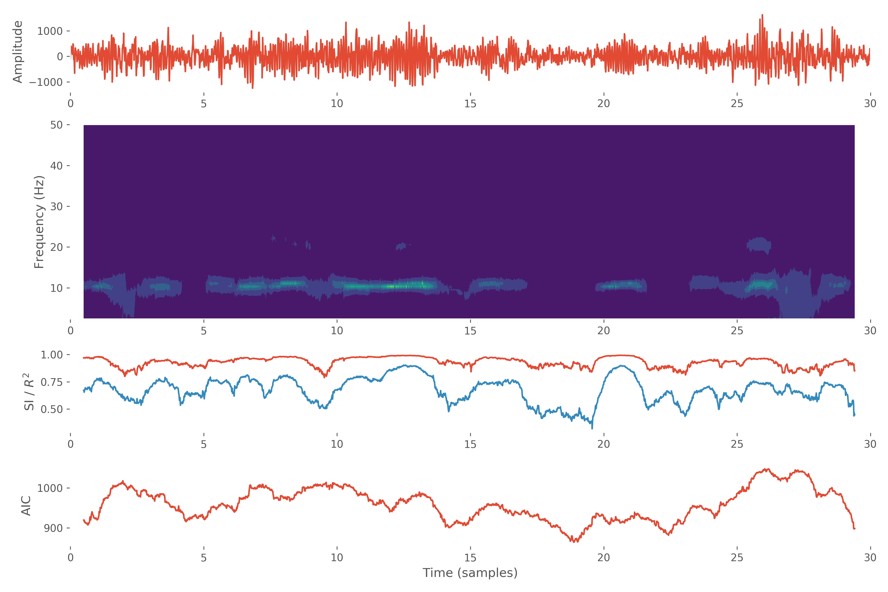
We will now produce a composite plot which illustrates how the behaviour of the system evolves over time. We are going to limit ourselves to the first 10000 data points and windows.
f1, axes = plt.subplots(nrows=5, ncols=1, figsize=(12, 8))
On the top row, we plot our data.
plt.subplot(5, 1, 1)

plt.plot(time_vect, X[0, :, 0])

plt.xlim(0, 30)
plt.grid(True)

plt.ylabel('Amplitude')
On the next two rows, we plot our transfer function for the first 10000 windows:
plt.subplot(5, 1, (2, 3))

plt.contourf(model_time_vect, F.freq_vect[3:], np.sqrt(np.abs(F.PSD[0, 0, 3:, :])))

plt.xlim(0, 30)
plt.grid(True)

plt.ylabel('Frequency (Hz)')
Underneath the transfer function, we examine the stability index (in red) and the \(R^2\) value (in blue):
plt.subplot(5, 1, 4)

plt.plot(model_time_vect, D.SI)

plt.plot(model_time_vect, D.R_square)

plt.xlim(0, 30)
plt.grid(True)

plt.ylabel('SI / $R^2$')
On the bottom row, we plot the AIC value for each of the models:
plt.subplot(5, 1, 5)

plt.plot(model_time_vect, D.AIC)

plt.xlim(0, 30)
plt.grid(True)

plt.xlabel('Time (samples)')

plt.ylabel('AIC')
Finally, we can look at our overall figure:
f1.tight_layout()

f1.show()