Tutorial 3 - Fitting real univariate data¶

In the previous two tutorials we set up our system using the polynomial representation. In most cases, we will want to learn the parameters of our model from real data. In this section, we cover how this is done.

We will be using some data from a single MEG Virtual Electrode reconstruction. The data has been down-sampled from the original sampling rate for the purposes of demonstration and ease of analysis.

We start with some imports and finding the location of our example data:

from os.path import join
import numpy as np
import matplotlib.pyplot as plt

from sails import find_example_path, root_plot, model_from_roots

plt.style.use('ggplot')

ex_dir = find_example_path()

The original MEG data was sampled at 2034.51Hz and has been down-sampled by 24 times giving us a sampling rate of just under 85Hz. The data has also been Z-scored. The data is stored in an HDF5 file in the example data directory as meg_single.hdf5; the data is stored as the dataset X.

import h5py

sample_rate = 2034.51 / 24

nyq = sample_rate / 2.

freq_vect = np.linspace(0, nyq, 64)

X = h5py.File(join(ex_dir, 'meg_single.hdf5'), 'r')['X'][...]

print(X.shape)

(1, 30157, 1)

The form of the data for the fitting routines is (nsignals, nsamples, ntrials). In the current case, we are performing a univariate analysis so we only have one signal. We have just over 30,000 data points and one one trial.

We are now in a position to set up our model. We will use the Vieira-Morf algorithm to fit our model, and fit a model of order 19 using the delay_vect argument. We will discuss model order selection in a later tutorial.

from sails import VieiraMorfLinearModel

delay_vect = np.arange(20)

m = VieiraMorfLinearModel.fit_model(X, delay_vect)

print(m.order)

We can now compute some diagnostics in order to check that our model looks sensible. We can start by looking at the R-squared value:

diag = m.compute_diagnostics(X)

print(diag.R_square)

0.41148872414

We can see that we are explaining just over 40% of the variance with our model which, given that we are modelling human MEG data collected over roughly 6 minutes, is reasonable.

The diagnostics class also gives us access to various other measures:

print(diag.AIC)

-25563.4038876

print(diag.BIC)

-25396.883104

print(diag.LL)

-25603.4038876

print(diag.DW)

[ 2.00103186]

print(diag.SI)

0.976853801393

print(diag.SR)

0.0663411856574

In turn, these are the Akaike Information Criterion (AIC), Bayesian Information Criterion (BIC), Log Likelihood (LL), Durbin-Watson coefficient (DW), Stability Index (SI) and Stability Ratio (SR). It is also possible to access the Percent Consistency (PC), although this is not computed by default due to it being memory intensive - you can compute this using the percent_consistency() routine.

As in our previous examples, we can extract our metrics and plot the transfer functions using both the Fourier and Modal methods as we have previously done:

from sails import FourierMvarMetrics, ModalMvarMetrics

F = FourierMvarMetrics.initialise(m, sample_rate, freq_vect)
F_H = F.H

M = ModalMvarMetrics.initialise(m, sample_rate, freq_vect)
M_H = M.modes.per_mode_transfer_function(sample_rate, freq_vect)

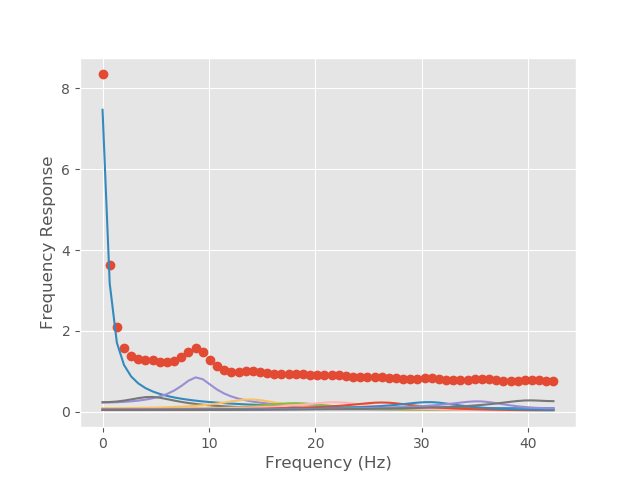
# Plot our fourier and modal spectra

f2 = plt.figure()

plt.plot(freq_vect, np.abs(F_H).squeeze(), 'o');
plt.plot(freq_vect, np.abs(M_H).squeeze());

plt.xlabel('Frequency (Hz)')
plt.ylabel('Frequency Response')

f2.show()

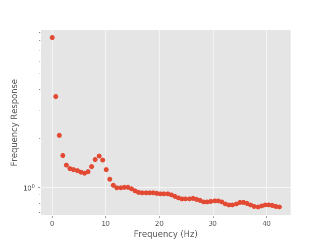
f3 = plt.figure()

plt.semilogy(freq_vect, np.abs(F_H).squeeze(), 'o');
plt.semilogy(freq_vect, np.abs(M_H).squeeze());

plt.xlabel('Frequency (Hz)')
plt.ylabel('Frequency Response')

f3.show()

In our previous examples, the model was defined by the structure of the polynomial, and we could analytically write down the form of the poles. In this example, we have learned the parameters from data. We may want to look at the plot of the system roots:

ax = M.modes.pole_plot()
ax.figure.show()

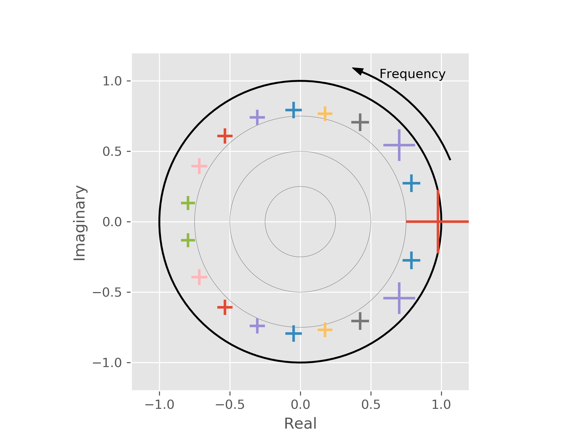
As previously, we can also go on to extract the magnitude of the eigenvalues and period of each of the modes:

ev = np.abs(M.modes.evals)

idx = [i[0] for i in M.modes.mode_indices]

print(ev[idx])

[[ 0.9768538 ]
 [ 0.88790649]
 [ 0.83392372]
 [ 0.82257801]
 [ 0.7869429 ]
 [ 0.79447331]
 [ 0.80151847]
 [ 0.81061091]
 [ 0.81709057]
 [ 0.80730369]]

print(M.modes.peak_frequency[idx])

[[  0.        ]
 [  8.88121272]
 [  4.51372792]
 [ 13.89286835]
 [ 18.15521077]
 [ 22.01471814]
 [ 26.47871083]
 [ 30.9324283 ]
 [ 35.59229698]
 [ 40.1740829 ]]

From this, we can see that the mode which primarily fits this data is an alpha mode at 8.9Hz.