Tutorial 2 - A more interesting oscillation

In this tutorial, we will extend our example to include oscillations on top of the background pink noise. We begin in the same way as with the previous tutorial.

import numpy as np
from sails import generate_pink_roots, root_plot, model_from_roots
import matplotlib.pyplot as plt

plt.style.use('ggplot')

sample_rate = 100
nyq = sample_rate / 2.

freq_vect = np.linspace(0, nyq, 64)

roots = generate_pink_roots(1)

We now add in energy at two frequencies and plot the poles.

roots[3:5] = roots[3:5]*1.1

roots[7:9] = roots[7:9]*1.1

ax = root_plot(roots)

ax.figure.show()

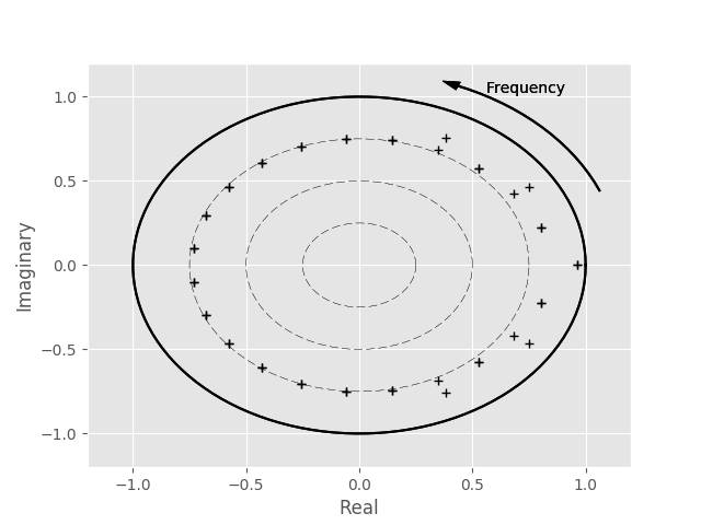
In this plot we can see that in addition to our pink noise mode on the x-axis (compare back to the equivalent plot in the first tutorial), we have two poles which now sit closer to the unit circle - these correspond to the additional energy which we have placed in the signal.

We can now continue to set up our model from our roots, generate the Fourier and Modal transfer functions and plot them as before:

from sails import FourierMvarMetrics, ModalMvarMetrics

m = model_from_roots(roots)

F = FourierMvarMetrics.initialise(m, sample_rate, freq_vect)
F_H = F.H

M = ModalMvarMetrics.initialise(m, sample_rate, freq_vect)
M_H = M.modes.transfer_function(sample_rate, freq_vect, sum_modes=True)

# Plot our fourier and modal spectra
f2 = plt.figure()

plt.plot(freq_vect, np.abs(F_H).squeeze(), 'o');
plt.plot(freq_vect, np.abs(M_H).squeeze());

plt.xlabel('Frequency (Hz)')
plt.ylabel('Frequency Response')

f2.show()

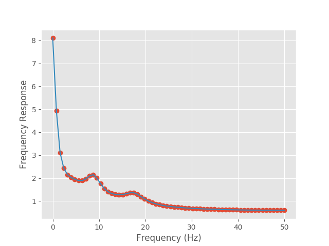
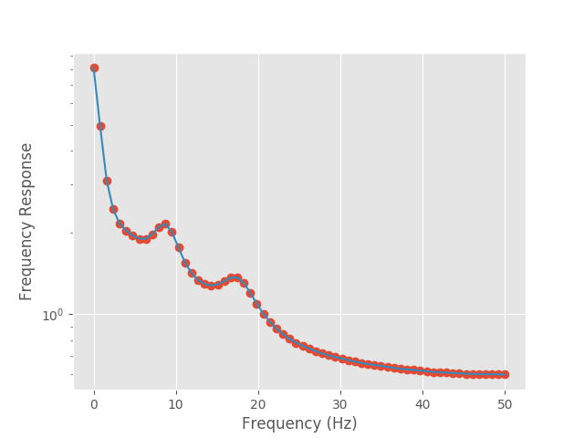
In comparison to our plot in the first tutorial, there are (as expected) two peaks in the Fourier transfer function at around 8Hz and 17Hz. We can also see that each of these two peaks has been extracted into a separate mode in the modal decomposition. This can be seen slightly more clearly by using a log scale for the y axis:

f3 = plt.figure()

plt.semilogy(freq_vect, np.abs(F_H).squeeze(), 'o');

plt.semilogy(freq_vect, np.abs(M_H).squeeze());

plt.xlabel('Frequency (Hz)')

plt.ylabel('Frequency Response')

f3.show()

We can also go on to extract the magnitude of the eigenvalues for each of the poles:

ev = np.abs(M.modes.evals)

Note that we have an eigenvalue for each of the poles, not each of the modes. As the eigenvalue will be identical for both of the poles in a given mode (where the mode consists of a pole pair), we can reduce down to examining one pole for each mode. To get the relevant indices, we can extract the information from the mode_indices property on the MvarModalDecomposition object. We can then extract other interesting pieces of information such as the period of the oscillation in the same way:

idx = [i[0] for i in M.modes.mode_indices]

print(ev[idx])

[[ 0.96393242]
 [ 0.83308007]
 [ 0.88077379]
 [ 0.78215297]
 [ 0.84650308]
 [ 0.7603617 ]
 [ 0.75345934]
 [ 0.74824023]
 [ 0.74435422]
 [ 0.73893252]
 [ 0.73980532]
 [ 0.74158676]]

print(M.modes.peak_frequency[idx])

[[  0.        ]
 [  4.37353106]
 [  8.83055516]
 [ 13.2106547 ]
 [ 17.56247546]
 [ 21.90065104]
 [ 26.23121568]
 [ 30.55715939]
 [ 34.88016321]
 [ 47.84046803]
 [ 43.52119577]
 [ 39.20127164]]

From this, we can see that the modes which fit our two oscillations are found at 8.8Hz and 17.6Hz.